Fast.ai Part 2 — Lecture 1 Object Detection

After David Uminsky, who is the Director of Data Institute, finished his welcome speech and called over Jeremy to get started with the course, Jeremy started the first class of Deep Learning Part 2 by thanking David, for making a course like this possible and available for many across the world. Though there is a lot to talk about this course and surely there is a need to spread the word about it so that many more people can get access to this course, I will spare that for a very-near-future post and for now I would like to thank David, Jeremy, Rachel and everyone else who made this course available for people from across the world.

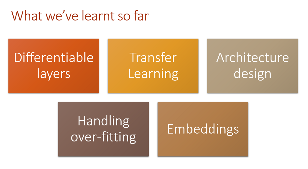
I finished taking the first lecture of Fast.ai Part 2 course on Deep Learning a few hours ago and I want to share what was taught and learnt from it through this post. If you are a Fast.ai student already, feel free to go through it and let me know what else could be added. Otherwise, make sure you go here and start taking the amazing lectures. Jeremy gave a quick review of few of the key takeaways from Part 1 of the course. He talked about how Deep Learning is so much about differentiable functions and mentioned Yann Lecun’s statement about Deep Learning - “ Deep Learning est mort. Vive Differentiable Programming!”(Click here for the original post).

Transfer Learning was present all throughout Part 1. We usually start with random weights and try to learn them(find their optimal values)so that the loss gets reduced. In the case of having weights that are already learnt(even if they are not totally relevant to the task at hand), it’s good to start with the learned weights(pre-trained models). If there is a model A that has learnt to perform a task U, even if it is only remotely close to another task V, the model can still be taken and fine-tuned by re-learning the last layers. This way the learning is quicker and doesn’t need as much data as getting started with random weights. CNN architecture, over-fitting and embedding were few other main concepts that were discussed in Part 1. Adding more data, data augmentation, batch normalisation, regularisation using weight decay and drop-out, reducing the complexity of the model(more complex models have more layers and parameters, so they don’t often generalise well for unseen data) are ways to avoid over-fitting.

One of the best parts of Fast.ai is the tips and suggestions you receive from the class. Don’t think too much about model over-fitting initially. It’s something that should be worried about when you want to optimize the model, not when you are creating it. There will be flaws in the code that you come across and that’s not unusual. So when something doesn’t work as expected, remember this as one of the possibilities(may not always be the case though!).Whether it’s Fast.ai or any other forum, don’t be afraid/shy to ask questions. But before you do, make sure you give it a try.

Jupyter notebooks are interactive and easy to run. So take the notebook that has the code for each lecture, start from the first cell and keep executing one after the other and see how things work. Copy & Paste whenever you need to. When you face some issues with the same code that worked in the lecture, run to the forum and shoot the questions!!

Above are some of the must DON’Ts. Simply going through each cell of the code might help you see the results of what each cell does. But it doesn’t help in getting better at coding the model or knowing the approach to solving even a slightly different task. For a much better approach, check this wiki post. It’s a very good practice to read papers, understand them, try and explain it in plain language for others through blogs and also try and implement them. This also makes one realise how, easy to understand things are made complicated in an attempt to gather theoretical knowledge. I laughed when Jeremy was saying all this. If you have taken Part 1 already, you must be aware of such harmless, fun pokes that Jeremy makes once in a while. I call them The Jeremy Jokes!

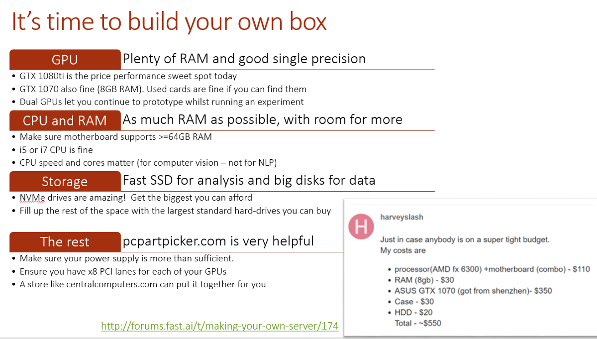
Deep Learning models usually consume a lot of data and need more than decent computational power. Typical CPUs can’t afford such computational demand. To run such models on large datasets, it’s better to go with cloud computing services or to build your own GPU box. The below picture can be helpful with setting up your own GPU box:

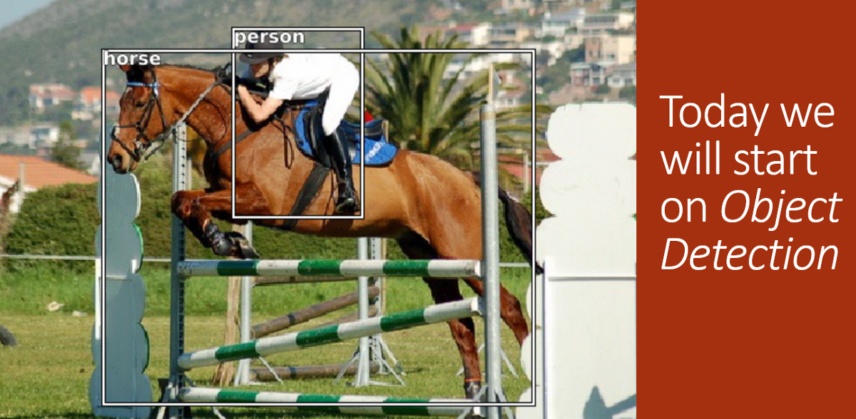
It’s time for Object Detection! I guess one need not explain what it is. But still for the note-sake, given an image with one or more objects, object detection is the process of locating, classifying and labelling objects of different classes/categories in the image. It is obvious that it is close to Computer Vision. To perform object detection, we chose the Pascal Visual Object Classes dataset. The Pascal VOC Project ran challenges for several years(2005–2012)evaluating performance on object class recognition. Each year’s datasets are available to download. In the lecture notebook, we used the data that was derived from 2007 challenge. Besides the images, another important part of this dataset is the annotations which contain the actual information about what all objects are present in each image, the classes of each object and the bounding box. Since this annotation information is in .xml format in the original dataset, we used the derived dataset which has the same data in .json format and is easier to use. More details about the dataset and project can be found here.

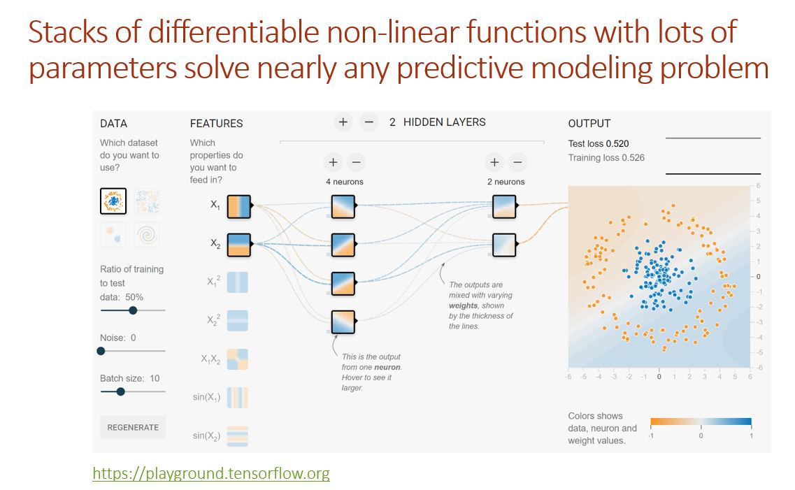
Jeremy showed a slide at the beginning of the lecture that had TensorFlow playground. I came across the same when I was going through Machine Learning crash course which Google made available to everyone a few weeks ago. If you haven’t taken it yet, I would recommend you to go through it since it explains many of the Machine Learning concepts quite well. You can find more about the course here.

Object detection varies depending on what you want to achieve. If it’s about recognising faces in a picture, you want to find and label all of them. When searching for a specific object, you want the model to filter it out from the rest. In the first lecture of Part 2, we start with detecting the largest object in an image and classifying it. This gives us a good starting point for object detection. For step 1, we find the largest object in the image, classify the image(give it a label) and draw a bounding box around it.

I have added notes, a bit of explanation and coding tips that Jeremy shared, in the lecture’s Jupyter notebook which you can access from here. We did the first step of object detection which is finding the largest object in the image, labelling it and then setting a bounding box around it. Visual Studio Code is the recommended editor to browse and modify the code. Jeremy shared few commonly used shortcuts on VSC. It was also showed how a debugger can be very handy. The one that’s used in the lecture was pdb, Python Debugger. I haven’t used these tools until now. Considering how handy and useful they could be, I started giving them a try. Maybe I could write a post on them in the future!

Click here for the lecture’s notebook with added notes and explanation.

It’s really exciting to be a Fast.ai International Fellow. Attending live lectures and being part of the amazing forum could make a lot of difference. I would like to end by sharing something which Jeremy talked about in this lecture. In theory, we learn about architectures, activation functions, loss functions, gradients etc and form an intuition. It’s a totally different thing to try it out and practice. In the process, things may not always work, especially in the beginning. But what’s important is to not give up. As long as learning motivates you, you should keep trying and learning.

I will keep updating the post if I find anything useful and relevant to this lecture. Don’t hesitate to leave your response. Let me know what you think about this post. Thanks for reading and happy learning!!!